Projection Matrices
What are projection matrices?
One-Dimensional Projections
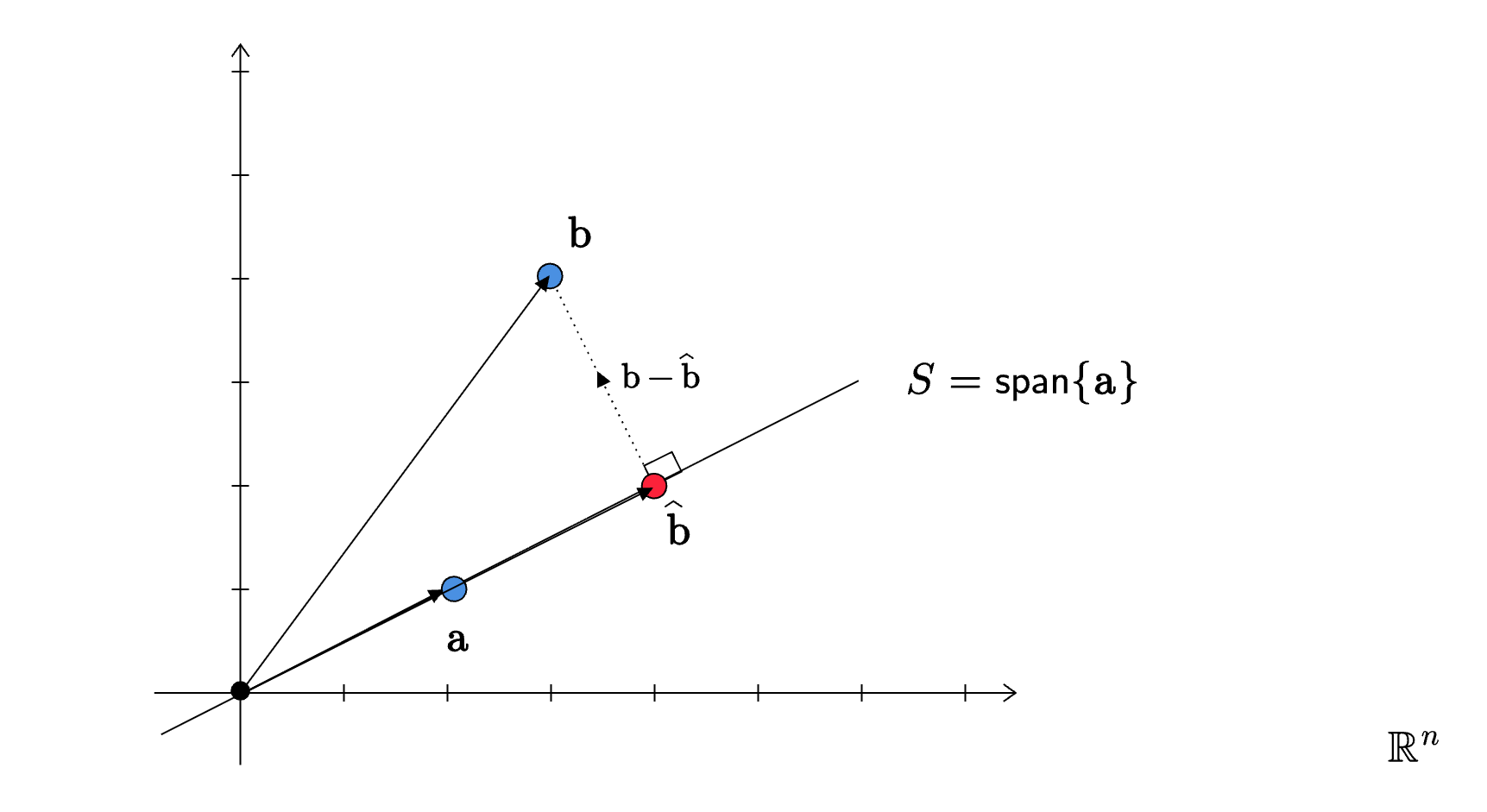
Consider a non-zero vector \(\mathbf{a} \in \mathbb{R}^{n}\). We have already seen what it means to project any vector \(\mathbf{b} \in \mathbb{R}^{n}\) onto \(S=\text{span}\{\mathbf{a}\}\). The projection is given by:
\[ \widehat{\mathbf{b}} =\frac{\mathbf{b}^{T}\mathbf{a}}{\mathbf{a}^{T}\mathbf{a}}\mathbf{a} \]
Let us quickly revisit the proof. The projection of \(\mathbf{b}\) onto \(S\) is a vector \(\widehat{\mathbf{b}}\) in \(S\) that is closest to \(\mathbf{b}\). If we set \(\widehat{\mathbf{b}} =\alpha \mathbf{a}\), then, we have to solve the following problem:
\[ \underset{\widehat{\mathbf{b}} \in S}{\min} \ ||\mathbf{b} -\widehat{\mathbf{b}} ||^{2} \]
Expanding the function:
\[ \begin{aligned} ||\mathbf{b}-\widehat{\mathbf{b}} ||^{2} & =||\mathbf{b}-\alpha \mathbf{a}||^{2}\\ & \\ & =( \mathbf{b}-\alpha \mathbf{a})^{T}( \mathbf{b}-\alpha \mathbf{a})\\ & \\ & =\alpha ^{2}\left( \mathbf{a}^{T} \mathbf{a}\right) -2\alpha \left( \mathbf{b}^{T} \mathbf{a} \right) +\left( \mathbf{b}^{T} \mathbf{b}\right) \end{aligned} \]
With the help of some calculus, we can show that the minimum value of the above expression occurs when:
\[ \alpha =\frac{\mathbf{b}^{T} \mathbf{a}}{\mathbf{a}^{T} \mathbf{a}} \]
Therefore, the projection of \(\mathbf{b}\) onto \(S=\text{span}\{\mathbf{a}\}\) is:
\[ \widehat{\mathbf{b}} =\frac{\mathbf{b}^{T}\mathbf{a}}{\mathbf{a}^{T}\mathbf{a}}\mathbf{a} \]
Geometrically, \(\mathbf{b} -\widehat{\mathbf{b}}\) is orthogonal to \(S = \text{span}\{\mathbf{a}\}\). We can summarize all this in the following figure:
The projection matrix is a square matrix of shape \(n \times n\) that projects any vector in \(\mathbb{R}^{n}\) onto \(\text{span}\{\mathbf{a}\}\). This is given by:
\[ \mathbf{P} =\frac{\mathbf{aa}^{T}}{\mathbf{a}^{T}\mathbf{a}} \]
The projection matrix in this case has rank \(1\). Besides, we also note the following important properties that it possesses:
\(\mathbf{P}^{2} =\mathbf{P}\)
\(\mathbf{P}^{T} =\mathbf{P}\)
Matrices that satisfy \(\mathbf{P}^{2} =\mathbf{P}\) are called idempotent. The projection matrix in this special case of one-dimensional projections seems to be symmetric and idempotent. In fact, it is true of all projection matrices as we will soon show.
Projections in General
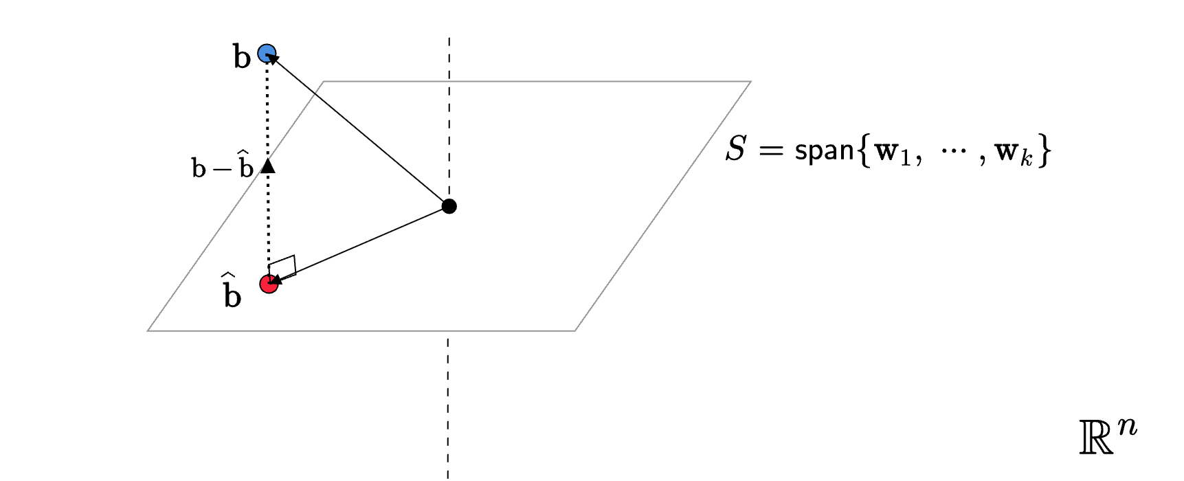
Let us now try to generalize this idea. Consider a \(k\) dimensional subspace \(S\) in \(\mathbb{R}^{n}\), with \(k< n\). We wish to project a vector \(\mathbf{b}\in \mathbb{R}^{n}\) onto the subspace \(S\) and determine the projection matrix associated with this subspace. How do we go about doing this?
Optimization Problem
The study of projections and projection matrices is greatly simplified if we work with orthonormal bases. So the first thing we will do is to declare an orthonormal basis for \(S\). Since \(S\) is \(k\)-dimensional, this basis would have size \(k\). Therefore:
\[ S=\text{span}\{\mathbf{w}_{1} ,\cdots ,\mathbf{w}_{k}\} \]
where, \(\mathbf{w}_{i} \perp \mathbf{w}_{j}\) for \(i\neq j\) and \(||\mathbf{w}_{i} ||=1\). Now, any collection of linearly independent vectors in \(\mathbb{R}^{n}\) can be extended to form a basis. In fact, we can extend any subset of non-zero orthonormal vectors in \(\mathbb{R}^{n}\) to an orthonormal basis for it. Though we won’t be proving this here, we can safely posit the existence of such a basis:
\[ \beta=\{\mathbf{w}_{1} ,\cdots ,\mathbf{w}_{k} ,\mathbf{w}_{k+1} ,\cdots ,\mathbf{w}_{n}\} \]
\(\beta\) is an orthonormal basis for \(\mathbb{R}^{n}\). With this preliminary setup done, let us go back to the question of projecting vectors onto \(S\). We have \(\mathbf{b} \in \mathbb{R}^{n}\). Since \(\beta\) is an orthonormal basis for \(\mathbb{R}^{n}\), we can express \(\mathbf{b}\) as the following unique linear combination:
\[ \mathbf{b} =\left(\mathbf{b}^{T}\mathbf{w}_{1}\right)\mathbf{w}_{1} +\cdots +\left(\mathbf{b}^{T}\mathbf{w}_{n}\right)\mathbf{w}_{n} \]
Next, the projection of \(\mathbf{b}\) onto \(S\) is a vector \(\widehat{\mathbf{b}} \in S\) that is closest to \(\mathbf{b}\). This is equivalent to solving the following optimization problem:
\[ \underset{\widehat{\mathbf{b}} \in S}{\min} \ ||\mathbf{b} -\widehat{\mathbf{b}} ||^{2} \]
Since \(\widehat{\mathbf{b}} \in S\), we can express it uniquely as:
\[ \widehat{\mathbf{b}} =\alpha _{1}\mathbf{w}_{1} +\cdots +\alpha _{k}\mathbf{w}_{k} \]
First, let us compute \(\mathbf{b} -\widehat{\mathbf{b}}\):
\[ \begin{aligned} \mathbf{b} -\widehat{\mathbf{b}} & =\left(\mathbf{b}^{T}\mathbf{w}_{1} -\alpha _{1}\right)\mathbf{w}_{1} +\cdots +\left(\mathbf{b}^{T}\mathbf{w}_{k} -\alpha _{k}\right)\mathbf{w}_{k}\\ & +\left(\mathbf{b}^{T}\mathbf{w}_{k+1}\right)\mathbf{w}_{k+1} +\cdots +\left(\mathbf{b}^{T}\mathbf{w}_{n}\right)\mathbf{w}_{n} \end{aligned} \]
It follows that \(||\mathbf{b} -\widehat{\mathbf{b}} ||^{2}\) is:
\[ \begin{aligned} ||\mathbf{b} -\widehat{\mathbf{b}} ||^{2} & =\left(\mathbf{b}^{T}\mathbf{w}_{1} -\alpha _{1}\right)^{2} +\cdots +\left(\mathbf{b}^{T}\mathbf{w}_{k} -\alpha _{k}\right)^{2}\\ & +\left(\mathbf{b}^{T}\mathbf{w}_{k+1}\right)^{2} +\cdots +\left(\mathbf{b}^{T}\mathbf{w}_{n}\right)^{2} \end{aligned} \]
Note that the \(\alpha _{i}\)-s are the variables of the optimization problem. It becomes clear that \(||\mathbf{b}-\widehat{\mathbf{b}}||^{2}\) attains its minimum when \(\alpha _{i} =\mathbf{b}^{T}\mathbf{w}_{i}\) for \(1\leqslant i\leqslant k\). Therefore, we end up with:
\[ \widehat{\mathbf{b}} =\left(\mathbf{b}^{T}\mathbf{w}_{1}\right)\mathbf{w}_{1} +\cdots +\left(\mathbf{b}^{T}\mathbf{w}_{k}\right)\mathbf{w}_{k} \]
We now see that \(\mathbf{b}\) can be expressed as:
\[ \begin{aligned} \mathbf{b} & =\left(\mathbf{b}^{T}\mathbf{w}_{1}\right)\mathbf{w}_{1} +\cdots +\left(\mathbf{b}^{T}\mathbf{w}_{k}\right)\mathbf{w}_{k}\\ & \ \ \ +\left(\mathbf{b}^{T}\mathbf{w}_{k+1}\right)\mathbf{w}_{k+1} +\cdots +\left(\mathbf{b}^{T}\mathbf{w}_{n}\right)\mathbf{w}_{n}\\ & =\widehat{\mathbf{b}} +\widehat{\mathbf{b}}_{\perp } \end{aligned} \]
Though we didn’t begin with this, what we have shown is that \(\widehat{\mathbf{b}}_{\perp } =\mathbf{b} -\widehat{\mathbf{b}}\) is orthogonal to \(S\). In other words, to obtain the projection of \(\mathbf{b}\) onto \(S\), we just need to retain the first \(k\) components when \(\mathbf{b}\) is expressed using the basis \(\beta\), where we must take care to note that \(\beta\) is obtained by extending an orthonormal basis of the subspace \(S\) to a basis for \(\mathbb{R}^{n}\).
Projection Matrix
We can now rearrange the RHS of \(\widehat{\mathbf{b}}\) by introducing matrices. Letting \(\mathbf{w}_{1} ,\cdots ,\mathbf{w}_{k}\) be the columns of a matrix \(\mathbf{W}\), we have:
\[ \mathbf{W} =\begin{bmatrix} | & & |\\ \mathbf{w}_{1} & \cdots & \mathbf{w}_{k}\\ | & & | \end{bmatrix} \]
From this, we observe that \(\mathbf{W}^{T}\mathbf{b}\) contains the coordinates of the vector \(\widehat{\mathbf{b}}\) in the basis \(\beta\):
\[ \begin{aligned} \mathbf{W}^{T}\mathbf{b} & =\begin{bmatrix} - & \mathbf{w}_{1}^{T} & -\\ & \vdots & \\ - & \mathbf{w}_{k}^{T} & - \end{bmatrix}\mathbf{b}\\ & \\ & =\begin{bmatrix} \mathbf{w}_{1}^{T}\mathbf{b}\\ \vdots \\ \mathbf{w}_{k}^{T}\mathbf{b} \end{bmatrix}\\ & \\ & =\begin{bmatrix} \mathbf{b}^{T}\mathbf{w}_{1}\\ \vdots \\ \mathbf{b}^{T}\mathbf{w}_{k} \end{bmatrix} \end{aligned} \]
Finally, \(\widehat{\mathbf{b}}\) itself can be expressed as follows:
\[ \begin{aligned} \widehat{\mathbf{b}} & =\begin{bmatrix} | & & |\\ \mathbf{w}_{1} & \cdots & \mathbf{w}_{k}\\ | & & | \end{bmatrix}\begin{bmatrix} \mathbf{b}^{T}\mathbf{w}_{1}\\ \vdots \\ \mathbf{b}^{T}\mathbf{w}_{k} \end{bmatrix}\\ & \\ & =\mathbf{WW}^{T}\mathbf{b} \end{aligned} \]
We can now extract the projection matrix onto the subspace \(S\) as:
\[ \mathbf{P} =\mathbf{WW}^{T} \]
where the columns of \(\mathbf{W}\) form an orthonormal basis for \(S\). Let us now take a quick look at the shapes of the matrices involved:
\(\mathbf{W}\) is \(n\times k\)
\(\mathbf{W}^{T}\) is \(k\times n\)
\(\mathbf{P}\) is \(n\times n\)
Properties
Unit Rank Decomposition, Column space, Nullspace
\(\mathbf{P}\) can be expressed as the sum of \(k\) rank-1 matrices:
\[ \mathbf{P} =\mathbf{w}_{1}\mathbf{w}_{1}^{T} +\cdots +\mathbf{w}_{k}\mathbf{w}_{k}^{T} \]
Using this we can show that:
the column space of \(\mathbf{P}\) is \(S\), that is, \(\begin{aligned} \mathcal{R}(\mathbf{P}) & =S \end{aligned}\)
the nullspace of \(\mathbf{P}\) is \(S^{\perp }\), that is, \(\begin{aligned} \mathcal{N}(\mathbf{P}) & =S^{\perp } \end{aligned}\)
It follows that rank of \(\mathbf{P}\) is \(k\) and its nullity is \(n - k\). Putting this in another way, for any vector \(\mathbf{x} \in S\), \(\mathbf{Px} =\mathbf{x}\) and for any vector \(\mathbf{x} \in S^{\perp }\), we have \(\mathbf{Px} =\mathbf{0}\). Therefore, we see that for a projection matrix, its column space is orthogonal to its nullspace. Geometrically what we see here makes sense. All vectors in \(S\) are left undisturbed by \(\mathbf{P}\) since they are already in \(\mathbf{P}\). This is what \(\mathbf{Px} =\mathbf{x}\) means for \(\mathbf{x} \in S\). Also, for vectors orthogonal to \(S\), those that lie in \(S^{\perp }\), \(\mathbf{Px} =\mathbf{0}\). They collapse to the origin.
Symmetry and Idempotence
First, we observe that \(\mathbf{P}\) is symmetric. Also, note that \(\mathbf{W}^{T}\mathbf{W}\), the identity matrix of shape \(k\times k\). This is because, the \(( ij)^{\text{th}}\) element is just the dot product between the orthonormal pair \(\mathbf{w}_{i}\) and \(\mathbf{w}_{j}\):
\[ \begin{aligned} \mathbf{W}^{T}\mathbf{W} & =\begin{bmatrix} - & \mathbf{w}_{1}^{T} & -\\ & \vdots & \\ - & \mathbf{w}_{k}^{T} & - \end{bmatrix}\begin{bmatrix} | & & |\\ \mathbf{w}_{1} & \cdots & \mathbf{w}_{k}\\ | & & | \end{bmatrix}\\ & \\ & =\begin{bmatrix} & \vdots & \\ \cdots & \mathbf{w}_{i}^{T}\mathbf{w}_{j} & \cdots \\ & \vdots & \end{bmatrix}\\ & \\ & =\mathbf{I} \end{aligned} \]
With this, we can conclude that \(\mathbf{P}\) is idempotent:
\[ \begin{aligned} \mathbf{P}^{2} & =\left(\mathbf{WW}^{T}\right)\mathbf{WW}^{T}\\ & \\ & =\mathbf{W}\left(\mathbf{W}^{T}\mathbf{W}\right)\mathbf{W}^{T}\\ & \\ & =\mathbf{WW}^{T}\\ & \\ & =\mathbf{P} \end{aligned} \]
Projection on \(S\) and \(S^{\perp }\)
For the next observation, we first note that any vector \(\mathbf{x}\mathbb{\in R}^{n}\) can be expressed uniquely as the sum of two vectors, one of which is in \(S\) and the other being perpendicular to \(S\):
\[ \mathbf{x} =\mathbf{x}_{S} +\mathbf{x}_{S^{\perp }} \]
To see why this is true, let us get back to the basis \(\beta\) to represent \(\mathbf{x}\):
\[ \begin{aligned} \mathbf{x} & =\left(\mathbf{x}^{T}\mathbf{w}_{1}\right)\mathbf{w}_{1} +\cdots +\left(\mathbf{x}^{T}\mathbf{w}_{n}\right)\mathbf{w}_{n}\\ & \\ \Longrightarrow \mathbf{x} & =\left(\mathbf{x}^{T}\mathbf{w}_{1}\right)\mathbf{w}_{1} +\cdots +\left(\mathbf{x}^{T}\mathbf{w}_{k}\right)\mathbf{w}_{k}\\ & \ \ +\left(\mathbf{x}^{T}\mathbf{w}_{k+1}\right)\mathbf{w}_{k+1} +\cdots +\left(\mathbf{x}^{T}\mathbf{w}_{n}\right)\mathbf{w}_{n} \end{aligned} \]
Notice that the first part of the RHS is in \(S\) while the second part is in \(S^{\perp }\). In fact, the first part is just the projection of \(\mathbf{x}\) on \(S\). The second part is the projection of \(\mathbf{x}\) on \(S^{\perp }\).
\[ \begin{aligned} \mathbf{x} & =\mathbf{Px} +(\mathbf{x} -\mathbf{Px})\\ & \\ \Longrightarrow \mathbf{x} & =\mathbf{Px} +(\mathbf{I} -\mathbf{P})\mathbf{x} \end{aligned} \]
Therefore, for any \(\mathbf{x} \in \mathbb{R}^{n}\), \(\mathbf{Px} \in S\) and \((\mathbf{I} -\mathbf{P})\mathbf{x} \in S^{\perp }\), are the projections of \(\mathbf{x}\) on the subspaces \(S\) and \(S^{\perp }\) respectively. Moreover, \(\mathbf{x}\) can be written as the sum of these these two vectors.
Length of Projection
This also leads us to the Pythagoras theorem. Since \(\mathbf{Px}\) and \((\mathbf{I} -\mathbf{P})\mathbf{x}\) are orthogonal, we have:
\[ \begin{aligned} ||\mathbf{x} ||^{2} & =||\mathbf{Px} ||^{2} +||(\mathbf{I} -\mathbf{P})\mathbf{x} ||^{2} \end{aligned} \]
From this we can infer following inequality:
\[ ||\mathbf{Px} ||\leqslant ||\mathbf{x} || \]
The length of the projection of a vector is at most the length of the vector. In other words, the base of a right triangle is always less than the hypotenuse. \(||\mathbf{Px} ||=||\mathbf{x} ||\) happens only when \(\mathbf{x}\) is already in \(S\).
Eigenvalues and Eigenvectors
Let us now compute the eigenvalues and eigenvectors of \(\mathbf{P}\). Let \(\mathbf{x} =\mathbf{x}_{S} +\mathbf{x}_{S^{\perp }}\) be an eigenvector of \(\mathbf{P}\) with eigenvalue \(\lambda\). Then, we have:
\[ \begin{array}{ c r l } & \mathbf{Px} & =\lambda \mathbf{x}\\ \Longrightarrow & \mathbf{P}(\mathbf{x}_{S} +\mathbf{x}_{S^{\perp }}) & =\lambda (\mathbf{x}_{S} +\mathbf{x}_{S^{\perp }})\\ \Longrightarrow & ( 1-\lambda )\mathbf{x}_{S} & =\lambda \mathbf{x}_{S^{\perp }} \end{array} \]
Since \(S\cap S^{\perp } =\{\mathbf{0}\}\), we see that \(( 1-\lambda )\mathbf{x}_{S} = \lambda \mathbf{x}_{S^{\perp }} =\mathbf{0}\). Solving each branch gives us two possibilities:
\(( 1,\mathbf{x})\) is an eigenpair for all \(\mathbf{x} \in S\) and \(\mathbf{x} \neq \mathbf{0}\)
\(( 0,\mathbf{x})\) is an eigenpair for all \(\mathbf{x} \in S^{\perp }\) and \(\mathbf{x} \neq \mathbf{0}\)
A number of inferences can be drawn from this:
\(1\) and \(0\) are the only eigenvalues of \(\mathbf{P}\)
\(E( 1) =S\) and \(E( 0) =S^{\perp }\) are the eigenspaces corresponding to these two eigenvalues
\(\mathbf{P}\) is orthogonally diagonalizable since it has an orthonormal basis of eigenvectors. This of course follows from the fact that \(\mathbf{P}\) is symmetric. But one needn’t invoke the spectral theorem to prove the fact in this particular case. In fact, we can now see that the decomposition of \(\mathbf{P}\) as the sum of \(k\) unit-rank matrices is nothing but the spectral decomposition of \(\mathbf{P}\):
\[ \begin{array}{ r l } \begin{array}{l} \mathbf{P} = \end{array} & 1\cdot \mathbf{w}_{1}\mathbf{w}_{1}^{T} +\cdots +1\cdot \mathbf{w}_{k}\mathbf{w}_{k}^{T}\\ & +\ 0\cdot \mathbf{w}_{k+1}\mathbf{w}_{k+1}^{T} +\cdots +0\cdot \mathbf{w}_{n}\mathbf{w}_{n}^{T} \end{array} \]
\[ \mathbf{P} =\mathbf{QDQ}^{T} \]
\[ \mathbf{D} =\begin{bmatrix} \mathbf{I}_{k\times k} & \mathbf{0}_{k\times ( n-k)}\\ \mathbf{0}_{( n-k) \times k} & \mathbf{0}_{( n-k) \times ( n-k)} \end{bmatrix} \]
Uniqueness of \(\mathbf{P}\)
One question still remains. What if we choose a different orthonormal basis to represent \(S\)? Will that yield a different projection matrix? Not really. There is only one projection matrix.
To prove this, let us assume that we have some other orthonormal basis for \(S\) so that \(S=\text{span}\left\{\mathbf{w}{_{1}}^{\prime } ,\cdots ,\mathbf{w}{_{k}}^{\prime }\right\}\). Extending this to a basis for \(\mathbb{R}^{n}\), we get \(\beta^{\prime } =\left\{\mathbf{w}{_{1}}^{\prime } ,\cdots ,\mathbf{w}{_{n}}^{\prime }\right\}\). Making the first \(k\) vectors as the columns of a matrix \(\mathbf{W}^{\prime }\), we can define a projection matrix for \(S\) as \(\mathbf{P}^{\prime } =\mathbf{W}^{\prime }\mathbf{W}{^{\prime }}^{T}\).
For \(\displaystyle 1\leqslant i\leqslant k\), we have:
\[ \begin{aligned} \mathbf{Pw}{_{i}}^{\prime } & =\mathbf{w}{_{i}}^{\prime }\\ \mathbf{P}^{\prime }\mathbf{w}{_{i}}^{\prime } & =\mathbf{w}{_{i}}^{\prime } \end{aligned} \Longrightarrow \mathbf{Pw}{_{i}}^{\prime } =\mathbf{P}^{\prime }\mathbf{w}{_{i}}^{\prime } \]
The first equality works because \(\displaystyle \mathbf{w}{_{i}}^{\prime } \in S\) and \(\displaystyle \mathbf{P}\) is a projection matrix for \(\displaystyle S\). The second equality works for the same reason. Alternatively, it also follows from the definition of \(\displaystyle \mathbf{P}^{\prime }\). For similar reasons, for \(\displaystyle k+1\leqslant i\leqslant n\), we have:
\[ \begin{aligned} \mathbf{Pw}{_{i}}^{\prime } & =\mathbf{0}\\ \mathbf{P}^{\prime }\mathbf{w}{_{i}}^{\prime } & =\mathbf{0} \end{aligned} \Longrightarrow \mathbf{Pw}{_{i}}^{\prime } =\mathbf{P}^{\prime }\mathbf{w}{_{i}}^{\prime } \]
Since \(\displaystyle \mathbf{P}\) and \(\displaystyle \mathbf{P}^{\prime }\) agree on all vectors in a basis \(\displaystyle \beta ^{\prime }\) for \(\displaystyle \mathbb{R}^{n}\), \(\displaystyle \mathbf{P} =\mathbf{P}^{\prime }\).
Equivalent Definitions
So far we have assumed the existence of a subspace \(S\) for which we have constructed a projection matrix. What about the reverse direction? If we have a matrix \(\mathbf{A}\), when can we say that it is the projection matrix for some subspace? To answer this question, we can work with the properties a projection matrix ought to have.
Recall that the final form of a projection matrix was \(\mathbf{WW}^{T}\) where the columns of \(\mathbf{W}\) are orthonormal. So we have one test for a projection matrix:
If a square matrix \(\mathbf{A}\) can be expressed as \(\mathbf{WW}^{T}\) where \(\mathbf{W}\) is an \(n\times k\) matrix with orthonormal columns, then \(\mathbf{A}\) is a projection matrix. Specifically, \(\mathbf{A}\) projects vectors in \(\mathbb{R}^{n}\) onto its column space.
This shouldn’t be too hard to see. The argument once again hinges on working with the orthonormal basis \(\beta=\{\mathbf{w}_{1} ,\cdots ,\mathbf{w}_{n}\}\), where the first \(k\) columns are drawn from \(\mathbf{W}\).
Next, recall that a projection matrix is idempotent and symmetric. Can we hope that all symmetric and idempotent matrices are projection matrices? In other words, are idempotence and symmetry sufficient conditions for a matrix to be a projection matrix? This is indeed the case.
If an \(n\times n\) matrix \(\mathbf{A}\) is idempotent and symmetric, then it is a projection matrix. Specifically, \(\mathbf{A}\) projects vectors in \(\mathbb{R}^{n}\) onto its column space.
We need to show two things.
Vectors that are in the column space should remain undisturbed under the projection.
Vectors orthogonal to the column space should collapse to zero under the projection.
Idempotence will help with the first test and symmetry with the second.
First, since \(\mathbf{A}^{2} =\mathbf{A}\), we have:
\[ \begin{array}{ c l l|c c } & \mathbf{A}^{2}\mathbf{x} & =\mathbf{Ax} & & \forall \mathbf{x} \in \mathbb{R}^{n}\\ \Longrightarrow & \mathbf{A}(\mathbf{Ax}) & =\mathbf{Ax} & & \forall \mathbf{x} \in \mathbb{R}^{n}\\ \Longrightarrow & \mathbf{Ay} & =\mathbf{y} & & \forall \mathbf{y} \in \mathcal{R}(\mathbf{A}) \end{array} \]
The last step shows that \(\mathbf{A}\) doesn’t disturb the elements in its column space. So it qualifies as a “general projection matrix”, one that brings all elements in \(\mathbb{R}^{n}\) onto a specific subspace while not disturbing elements that are native to that subspace.
What we need next is to see if \(\mathbf{A}\) is an orthogonal projection, that is, one that collapses vectors perpendicular to its column space to zero. This is where symmetry helps. Since \(\mathbf{A}\) is symmetric, its row space is equal to its column space. The nullspace of any matrix is orthogonal to the row space. But for a symmetric matrix, it is also orthogonal to the column space. Therefore, \(\mathbf{A}\) sends all vectors orthogonal to the column space to zero. This is enough to see that \(\mathbf{A}\) is a projection matrix!
Summary
A projection matrix \(\mathbf{P}\) is a matrix of shape \(n\times n\) that can be defined in any of the following ways, all of which are equivalent:
For all \(\mathbf{x} \in \mathbb{R}^{n}\), \(\mathbf{Px}\) is the projection of \(\mathbf{x}\) onto the column space of \(\mathbf{P}\), where by projection, we mean the vector \(\mathbf{Px}\) that minimizes \(||\mathbf{x} -\mathbf{Px} ||^{2}\).
\(\mathbf{P} =\mathbf{WW}^{T}\), where \(\mathbf{W}\) is a matrix of shape \(n\times k\) made up of orthonormal columns
\(\mathbf{P}\) is idempotent and symmetric.