\(\mathbf{Ax} = \mathbf{b}\)
How do we solve for \(\mathbf{x}\) in the equation \(\mathbf{Ax} =\mathbf{b}\)?
Column space
Now we come to the general form of a system of linear equations, \(\mathbf{Ax} =\mathbf{b}\). Let us recall the shapes of the objects involved:
\(\mathbf{A}\) is \(m \times n\)
\(\mathbf{x}\) is in \(\mathbb{R}^{n}\)
\(\mathbf{b}\) is in \(\mathbb{R}^{m}\)
First, we need to know if the system admits any solution at all. For this, we have to take a closer look at this system and see what it means:
\[ \begin{equation*} \begin{bmatrix} | & & |\\ \mathbf{a}_{1} & \cdots & \mathbf{a}_{n}\\ | & & | \end{bmatrix}\begin{bmatrix} x_{1}\\ \vdots \\ x_{n} \end{bmatrix} =\begin{bmatrix} b_{1}\\ \vdots \\ b_{m} \end{bmatrix} \end{equation*} \]
Here, \(\mathbf{a}_{1} ,\cdots ,\mathbf{a}_{n}\) are the columns of \(\mathbf{A}\). Recall that the product of a matrix and a vector can be interpreted as a linear combination of the columns of the matrix:
\[ \begin{equation*} x_{1}\mathbf{a}_{1} +\cdots +x_{n}\mathbf{a}_{n} =\mathbf{b} \end{equation*} \]
\(\mathbf{Ax} =\mathbf{b}\) has a solution if and only if \(\mathbf{b}\) can be expressed as a linear combination of the columns of \(\mathbf{A}\). Since the set of all linear combinations of the columns of \(\mathbf{A}\) is given by the \(\text{span} (\{\mathbf{a}_{1} ,\cdots ,\mathbf{a}_{n} \})\), the system is solvable if and only if \(\mathbf{b}\) belongs to \(\text{span}\left(\{\mathbf{a}_{1} ,\cdots ,\mathbf{a}_{n} \}\right)\).
The span of the columns of \(\mathbf{A}\) is a subspace of \(\displaystyle \mathbb{R}^{m}\) and is called the column space of the matrix \(\mathbf{A}\) and we denote it by \(\mathcal{R}(\mathbf{A})\):
\[ \mathcal{R} (\mathbf{A} )=\text{span} (\{\mathbf{a}_{1} ,\cdots ,\mathbf{a}_{n} \}) \]
We have now answered the question of when \(\mathbf{Ax} =\mathbf{b}\) is solvable. Since this is important, let us highlight it:
\(\mathbf{Ax}=\mathbf{b}\) has a solution if and only if \(\mathbf{b}\) is in the column space of \(\mathbf{A}\).
Augmented Matrix
Let us reuse the example from the previous unit:
\[ \begin{equation*} \begin{bmatrix} 1 & 0 & -1 & 0\\ 2 & 1 & 0 & 1\\ 3 & 1 & -1 & 1 \end{bmatrix}\begin{bmatrix} x_{1}\\ x_{2}\\ x_{3}\\ x_{4} \end{bmatrix} =\begin{bmatrix} b_{1}\\ b_{2}\\ b_{3} \end{bmatrix} \end{equation*} \]
We are back to the row-echelon form, but with the augmented matrix.
\[ \begin{equation*} \begin{bmatrix} 1 & 0 & -1 & 0 & b_{1}\\ 2 & 1 & 0 & 1 & b_{2}\\ 3 & 1 & -1 & 1 & b_{3} \end{bmatrix} \end{equation*} \]
Recall that the augmented matrix is formed by appending the column \(\mathbf{b}\) to the right of the matrix \(\mathbf{A}\). This is often denotes as \((\mathbf{A} | \mathbf{b})\), where the vertical separator indicates that we are augmenting the column \(\mathbf{b}\).
Why do we work with the augmented matrix now if we didn’t bother about it while solving \(\mathbf{Ax} = \mathbf{0}\)? Each row operation transforms a row into another row in a reversible manner. But rows are nothing but linear equations. So each row operation essentially transforms an equation into another form without disturbing the overall system. In this process, both sides of the equation have to undergo the same transformation. In a homogenous system, the RHS is always zero and remains immutable to any of the three row operations. The same can’t be said of the system we are studying.
Back to the augmented matrix:
\[ \begin{equation*} \begin{bmatrix} 1 & 0 & -1 & 0 & b_{1}\\ 2 & 1 & 0 & 1 & b_{2}\\ 3 & 1 & -1 & 1 & b_{3} \end{bmatrix} \end{equation*} \]
If we apply the same sequence of row operations as in the previous case, we get the row-reduced augmented matrix \((\mathbf{R}\ |\ \mathbf{c})\):
\[ \begin{equation*} \begin{bmatrix} 1 & 0 & -1 & 0 & b_{1}\\ 0 & 1 & 2 & 1 & b_{2} -2b_{1}\\ 0 & 0 & 0 & 0 & b_{3} -b_{1} -b_{2} \end{bmatrix} \end{equation*} \]
We can immediately see that the system has a solution if and only if the following condition is met:
\[ \begin{equation*} b_{3} -b_{1} -b_{2} =0 \end{equation*} \]
This gives us a useful rule to understand when a system of equations is consistent. Given its importance, let us frame it as a rule:
If the row reduced augmented matrix, \((\mathbf{R} \ |\ \mathbf{c})\), has a pivot in the last column, then the system is inconsistent.
Reintroducing the unknown vector \(\mathbf{x}\), the fruit of Gaussian elimination is the equivalent form \(\mathbf{R x} = \mathbf{c}\):
\[ \begin{equation*} \begin{bmatrix} 1 & 0 & -1 & 0\\ 0 & 1 & 2 & 1\\ 0 & 0 & 0 & 0 \end{bmatrix}\begin{bmatrix} x_{1}\\ x_{2}\\ x_{3}\\ x_{4} \end{bmatrix} =\begin{bmatrix} b_{1}\\ b_{2} -2b_{1}\\ 0 \end{bmatrix} \end{equation*} \]
Here, we assume that the system is consistent, so we let \(b_3 - b_1 - b_2 = 0\). Finally, we state the following result without proof:
\(\mathbf{x}^{\prime}\) is a solution to \(\mathbf{Ax} =\mathbf{b}\) if and only if \(\mathbf{x}^{\prime}\) is a solution to \(\mathbf{Rx} =\mathbf{c}\), where \((\mathbf{R} \ |\mathbf{\ c})\) is the matrix obtained from Gaussian elimination of the augmented matrix \((\mathbf{A}\ |\ \mathbf{b})\).
This allows us to work with the reduced system while temporarily forgetting the original system.
Particular Solution
If a solution exists, how do we find it? And what about all possible solutions? Let us now turn our attention to the system after row reduction:
\[ \mathbf{R} \mathbf{x} = \mathbf{c} \] First note that the set of pivot columns are linearly independent and form a basis for the column space of \(\mathbf{R}\). In the example we are working with, this is quite clear: \[ \begin{equation*} \mathcal{R} (\mathbf{R} )=\text{span}\left(\left\{\begin{bmatrix} 1\\ 0\\ 0 \end{bmatrix} ,\begin{bmatrix} 0\\ 1\\ 0 \end{bmatrix}\right\}\right) \end{equation*} \]
So, \(\mathbf{c}\) can be uniquely expressed as a linear combination of the columns of this basis. Let us call this a particular solution \(\mathbf{x}_{p}\). How do we find a particular solution \(\mathbf{x}_{p}\)? Coming back to the example we are working with:
\[ \begin{bmatrix} \mathbf{1} & 0 & -1 & 0\\ 0 & \mathbf{1} & 2 & 1\\ 0 & 0 & 0 & 0 \end{bmatrix}\begin{bmatrix} x_{1}\\ x_{2}\\ x_{3}\\ x_{4} \end{bmatrix} =\begin{bmatrix} b_{1}\\ b_{2} -2b_{1}\\ 0 \end{bmatrix} \]
The pivot variables are the multipliers of the pivot columns while the free variables are the multipliers of the non-pivot columns. Since our business is only with the pivot columns, we can set all free variables to zero with impunity and solve for the pivot variables. In this example, we would set \(x_3 = x_4 = 0\) and solve for \(x_1\) and \(x_2\). This gives us:
\[ \mathbf{x}_{p} =\begin{bmatrix} b_{1}\\ b_{2} -2b_{1}\\ 0\\ 0 \end{bmatrix} \]
Though this is the simplest way of obtaining a particular solution, it is by no means the only particular solution. Any solution to \(\mathbf{R x} = \mathbf{c}\) will qualify as a particular solution.
General Solution
We have found one solution. What about the rest? If \(\mathbf{x}_{p}\) is a particular solution and if know that \(\mathbf{A} \mathbf{x}_n = 0\) for some vector \(\mathbf{x}_n\) then it becomes clear that \(\mathbf{x}_{p} + \mathbf{x}_{n}\) is also a solution for the system. We also know that \(\mathbf{A} \mathbf{x}_n = 0\) if and only if \(\mathbf{x}_{n}\) is in the null space of \(\mathbf{A}\). Interestingly, it looks as though the homogenous system we studied in the previous document might actually play a helping hand here.
Description
If \(\mathbf{x}_{n}\) is some vector in the nullspace of \(\mathbf{A}\), then a general solution \(\mathbf{x}_{g}\) to the system can be expressed in this form:
\[ \begin{equation*} \mathbf{x}_{g} =\mathbf{x}_{p} +\mathbf{x}_{n} \end{equation*} \]
It may still not be clear why every solution should be of this form and we will prove this shortly. Before that, let us express the set of all solutions to a consistent system more formally:
\[ S = \mathbf{x}_p + \mathcal{N}(\mathbf{A}) \]
\(S\) is an affine space. Geometrically, an affine space is a subspace that is translated by some vector. In the simple setting of \(\mathbb{R}^{3}\), if the nullspace is a plane passing through the origin, then an affine space would be a plane parallel to it. Coming back to our context, the set of all solutions to \(\mathbf{Ax} = \mathbf{b}\) can be obtained by translating the nullspace of \(\mathbf{A}\) by a particular solution \(\mathbf{x}_p\).
Proof
We will show that this affine space is indeed the solution space. Let us call the set of all solutions \(S\). Now, pick up any element in the affine space: \[ \mathbf{x} = \mathbf{x}_p + \mathbf{x}_n \] where \(\mathbf{x}_n \in \mathcal{N}(\mathbf{A})\). We see that \(\mathbf{x}\) is a solution because: \[ \begin{equation*} \mathbf{Ax} =\mathbf{A} (\mathbf{x}_{p} +\mathbf{x}_{n} )=\mathbf{Ax}_{p} +\mathbf{Ax}_{n} =\mathbf{b} \end{equation*} \] We have shown that any arbitrary element of the affine space is also present in \(S\). In other words: \[ \mathbf{x}_p + \mathcal{N}(\mathbf{A}) \subset S \] Now we go the other way. Let \(\mathbf{x}\) be any element in \(S\). We can rewrite \(\mathbf{x}\) as: \[ \mathbf{x} = \mathbf{x}_p + (\mathbf{x} - \mathbf{x}_p) \] Now, note that \(\mathbf{x} - \mathbf{x}_p \in \mathcal{N}(\mathbf{A})\). This is because: \[ \mathbf{A}(\mathbf{x} - \mathbf{x}_p) = \mathbf{Ax} - \mathbf{Ax}_p = \mathbf{b} - \mathbf{b} = \mathbf{0} \] This shows that \(S \subset \mathbf{x}_p + \mathcal{N}(\mathbf{A})\). Thus we have the following beautiful result:
The set of all solutions to a consistent system \(\mathbf{Ax} = \mathbf{b}\) is the affine space \(\mathbf{x}_p + \mathcal{N}(\mathbf{A})\), where \(\mathbf{x}_{p}\) is a solution to the system.
Nature of Solutions
We have already seen that \(\displaystyle \mathbf{Ax} =\mathbf{b}\) has no solution or is inconsistent if \(\displaystyle \mathbf{b}\) is not in the column space of \(\displaystyle \mathbf{A}\). If \(\displaystyle \mathbf{b}\) is in the column space of \(\displaystyle \mathbf{A}\), then there are two possibilities. it could either have a unique solution or it could have infinitely many solutions. This depends on the nullspace of \(\displaystyle \mathbf{A}\). If the nullspace of \(\displaystyle \mathbf{A}\) is the trivial subspace \(\displaystyle \{\mathbf{0}\}\), then there is a unique solution. If not, the system has infinitely many solutions. This can be summarized in this neat graphical manner:
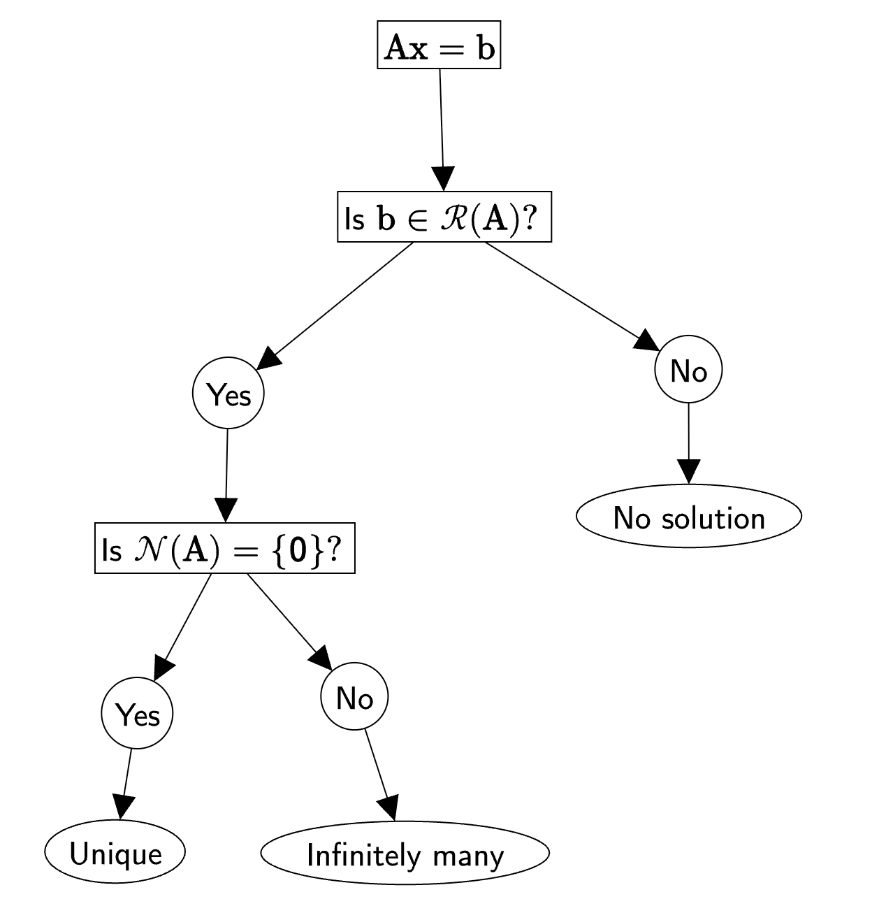
A new branch will be added to this when we study approximate solutions in the next document.
Column Space Revisited
Recall that we started this document with the attempt to look for coefficients \(\displaystyle x_{1} ,\cdots ,x_{n}\) such that the linear combination of the columns of \(\displaystyle \mathbf{A}\) with these coefficients would result in \(\displaystyle \mathbf{b}\):
\[ x_{1}\mathbf{a}_{1} +\cdots +x_{n}\mathbf{a}_{n} = \mathbf{b} \]
We did end up finding \(\displaystyle x_{1} ,\cdots ,x_{n}\). Curiously enough, we didn’t have to deal with the columns of \(\displaystyle \mathbf{A}\) as such, but with those of its cousin, the row-reduced matrix \(\displaystyle \mathbf{R}\). Specifically, we didn’t have to find the column space of \(\displaystyle \mathbf{A}\) explicitly. However, note that we did manage to find a basis for the column space of \(\displaystyle \mathbf{R}\) and hence its column space. Can we also extract the column space of \(\displaystyle \mathbf{A}\) somehow? The answer is yes.
We will state the answer without proof.
If \(\displaystyle \mathbf{R}\) is the RREF of \(\displaystyle \mathbf{A}\), then the columns in \(\displaystyle \mathbf{A}\) corresponding to the pivot columns of \(\displaystyle \mathbf{R}\) form a basis for the column space of \(\displaystyle \mathbf{A}\).
Back to our example:
\[ \begin{bmatrix} \textcolor[rgb]{0.99,0.13,0.23}{1} & \textcolor[rgb]{0.99,0.13,0.23}{0} & -1 & 0\\ \textcolor[rgb]{0.99,0.13,0.23}{2} & \textcolor[rgb]{0.99,0.13,0.23}{1} & 0 & 1\\ \textcolor[rgb]{0.99,0.13,0.23}{3} & \textcolor[rgb]{0.99,0.13,0.23}{1} & -1 & 1 \end{bmatrix}\rightarrow \begin{bmatrix} \textcolor[rgb]{0.99,0.13,0.23}{1} & \textcolor[rgb]{0.99,0.13,0.23}{0} & -1 & 0\\ \textcolor[rgb]{0.99,0.13,0.23}{0} & \textcolor[rgb]{0.99,0.13,0.23}{1} & 2 & 1\\ \textcolor[rgb]{0.99,0.13,0.23}{0} & \textcolor[rgb]{0.99,0.13,0.23}{0} & 0 & 0 \end{bmatrix} \]
The first two columns of \(\displaystyle \mathbf{R}\) are the pivot columns. Therefore, the first two columns of \(\displaystyle \mathbf{A}\) form a basis for the column space of \(\displaystyle \mathbf{A}\).
Summary
\(\mathbf{Ax} =\mathbf{b}\) is solvable if and only if \(\mathbf{b}\) is an element of the column space of \(\mathbf{A}\). A system that admits a solution is said to be consistent. Every solution to a consistent system of equations can be expressed as \(\mathbf{x}_{p} +\mathbf{x}_{n}\), where \(\mathbf{x}_{p}\) is a particular solution and \(\mathbf{x}_{n}\) is some vector in the nullspace of \(\mathbf{A}\). By varying \(\mathbf{x}_n\), we can get all possible solutions to the system.