Projections
Geometrically, what is the relationship between the approximation \(\mathbf{A}\widehat{\mathbf{x}}\) and the vector \(\mathbf{b}\)?
Setting
Recall that we solved the following system in the previous section:
\[ \mathbf{Ax} \approx \mathbf{b} \]
The best approximation is given by the solution to this system, also called the normal equations:
\[ (\mathbf{A}^{T}\mathbf{A} )\widehat{\mathbf{x}} =\mathbf{A}^{T}\mathbf{b} \]
Also, \(\displaystyle \mathbf{A\hat{x}}\) is the linear combination of the columns of \(\displaystyle \mathbf{A}\):
\[ \mathbf{A}\hat{\mathbf{x}} =\hat{x}_{1}\mathbf{a}_{1} +\cdots +\hat{x}_{n}\mathbf{a}_{n} \]
What we have with us is the best approximation to \(\displaystyle \mathbf{b}\) by a vector in the column space of \(\displaystyle \mathbf{A}\). The first thing to note is that both these vectors are in \(\displaystyle \mathbb{R}^{m}\). What happens if \(\displaystyle \mathbf{b}\) lies in the column space of \(\displaystyle \mathbf{A}\)? In such a situation, we can find values \(\displaystyle \hat{x}_{1} ,\cdots ,\hat{x}_{n}\) such that we can exactly construct \(\displaystyle \mathbf{b}\) as a linear combination of the columns of \(\displaystyle \mathbf{A}\). What we are more interested in, however, is the case where \(\displaystyle \mathbf{b}\) doesn’t lie on the column space. So we will stick to this scenario.
Moving forward, let us try to understand the geometric relationship between \(\displaystyle \mathbf{A\hat{x}}\) and \(\displaystyle \mathbf{b}\). To keep things simple, let us pitch our tent, \(\displaystyle \mathbb{R}^{2}\), with the following configuration:
\[ \begin{equation*} \mathbf{A} =\begin{bmatrix} 2 & 6\\ 1 & 3 \end{bmatrix} ,\ \mathbf{b} =\begin{bmatrix} 3\\ 4 \end{bmatrix} \end{equation*} \]
Back to Column space
We look for an approximation only when \(\mathbf{b}\) does not lie in the column space of \(\mathbf{A}\). So, first, we see what the column space is:
\[ \begin{equation*} \mathcal{R} (\mathbf{A} )=\text{span}\left(\left\{\begin{bmatrix} 2\\ 1 \end{bmatrix}\right\}\right) \end{equation*} \]
The second column of \(\mathbf{A}\) is just three times the first column. The rank of the matrix is \(1\). The column space of \(\mathbf{A}\) is a one-dimensional subspace of \(\mathbb{R}^{2}\) . Geometrically, what does this mean?

The column space is a line passing through the origin and the point \((2,1)\). Clearly, the vector \(\mathbf{b}\) does not lie in the column space of \(\mathbf{A}\). So, we are justified in looking for an approximation.
Projections: 2-dimensions
The key idea to remember is that the approximation is going to lie in the column space of \(\mathbf{A}\). What vector in \(\mathcal{R} (\mathbf{A} )\) is closest to to \(\mathbf{b}\)? Even before going there, what do we mean by closest? Recall that the Euclidean distance between the two vectors is our measure of the goodness of the approximation: smaller the distance, bettter the approximation. In our 2D case, this is nothing but the distance between the point \(\mathbf{b}\) and some point on the line \(\mathcal{R} (\mathbf{A} )\). The point on the line which is going to have the shortest distance is the foot of the perpendicular to the line. This is also called the orthogonal projection of \(\mathbf{b}\) onto the line.
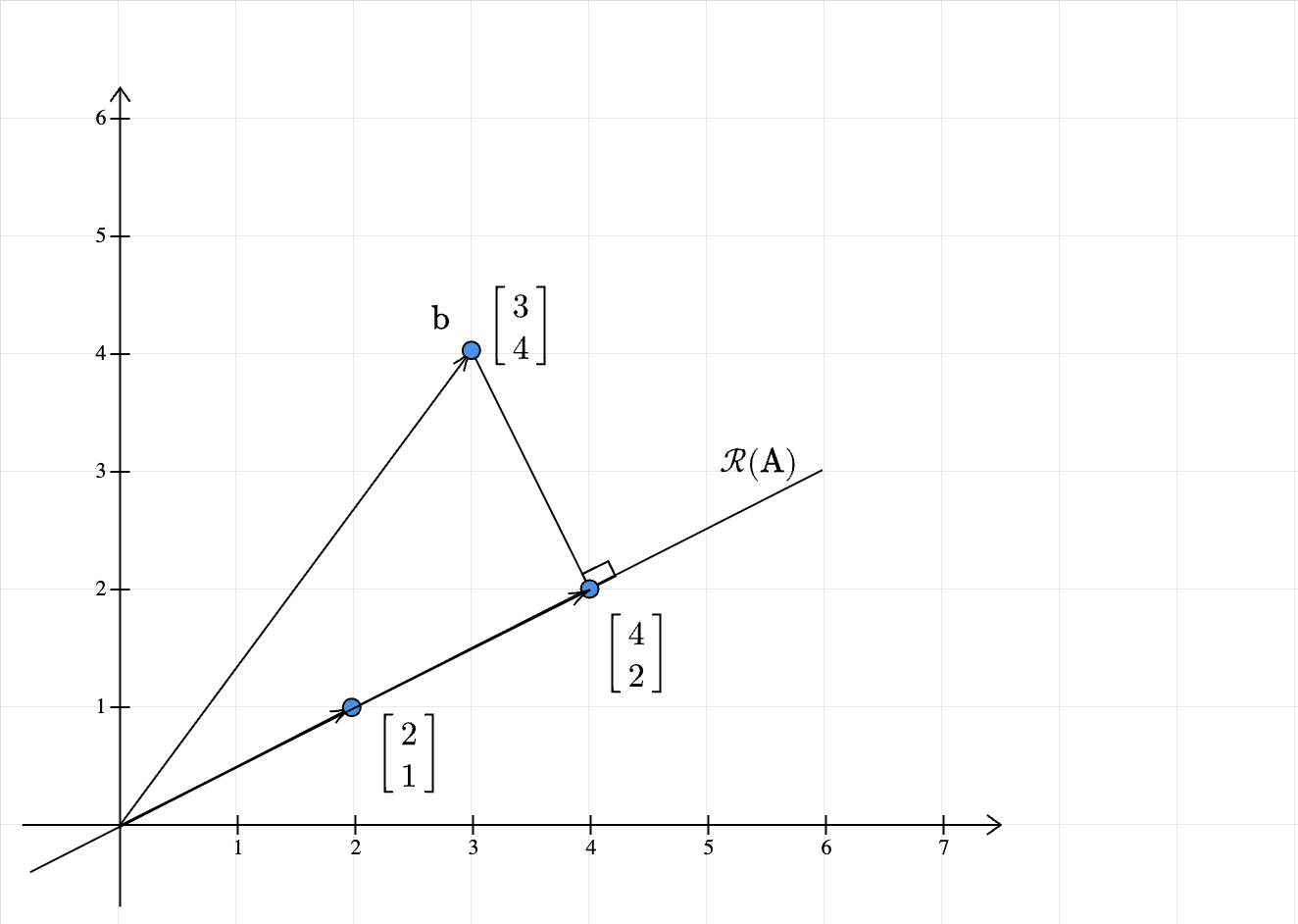
Geometric intuition therefore suggests that \(\mathbf{A}\widehat{\mathbf{x}} =\begin{bmatrix} 4\\ 2 \end{bmatrix}\).
Back to Normal Equations
Let us see if algebra agrees with geometry:
\[ \begin{equation*} \begin{aligned} (\mathbf{A}^{T}\mathbf{A} )\widehat{\mathbf{x}} & =\mathbf{A}^{T}\mathbf{b}\\ & \\ \begin{bmatrix} 2 & 1\\ 6 & 3 \end{bmatrix}\begin{bmatrix} 2 & 6\\ 1 & 3 \end{bmatrix}\begin{bmatrix} \widehat{x}_{1}\\ \widehat{x}_{2} \end{bmatrix} & =\begin{bmatrix} 2 & 1\\ 6 & 3 \end{bmatrix}\begin{bmatrix} 3\\ 4 \end{bmatrix}\\ & \\ \begin{bmatrix} 5 & 15\\ 15 & 45 \end{bmatrix}\begin{bmatrix} \widehat{x}_{1}\\ \widehat{x}_{2} \end{bmatrix} & =\begin{bmatrix} 10\\ 30 \end{bmatrix}\\ & \\ \begin{bmatrix} 1 & 3\\ 1 & 3 \end{bmatrix}\begin{bmatrix} \widehat{x}_{1}\\ \widehat{x}_{2} \end{bmatrix} & =\begin{bmatrix} 2\\ 2 \end{bmatrix} \end{aligned} \end{equation*} \]
We see that \(\mathbf{A}^{T}\mathbf{A}\) is singular. But thankfully, the system is still solvable. One such solution is:
\[ \begin{equation*} \widehat{\mathbf{x}} =\begin{bmatrix} -1\\ 1 \end{bmatrix} \end{equation*} \]
Therefore, the approximation is:
\[ \begin{equation*} \mathbf{A}\widehat{\mathbf{x}} =\begin{bmatrix} 2 & 6\\ 1 & 3 \end{bmatrix}\begin{bmatrix} -1\\ 1 \end{bmatrix} =\begin{bmatrix} 4\\ 2 \end{bmatrix} \end{equation*} \]
Algebra does agree with geometry!
Projections: higher dimensions
The main takeaway from the 2D case is this: the vector closest to \(\mathbf{b}\) in the column space of \(\mathbf{A}\) is its projection onto the column space of \(\mathbf{A}\). This can be extended to any higher dimensional space. First, we note that for a projection, the error vector is orthogonal to the column space of \(\mathbf{A}\):
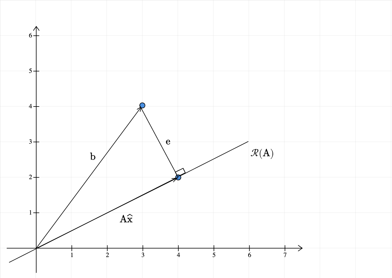
The error vector \(\mathbf{e}\) is:
\[ \begin{equation*} \mathbf{e} =\mathbf{b} -\mathbf{A}\widehat{\mathbf{x}} \end{equation*} \]
This is orthogonal to the column space of \(\mathbf{A}\). This is the same as saying that it is orthogonal to each column of \(\mathbf{A}\). If we let \(\mathbf{A}\) to be \([\mathbf{a}_{1} ,\cdots ,\mathbf{a}_{n} ]\). Then for \(1\leqslant i\leqslant n\):
\[ \begin{equation*} \mathbf{a}_{i}^{T}\mathbf{e} =0 \end{equation*} \]
This can be neatly expressed as:
\[ \begin{equation*} \mathbf{A}^{T}\mathbf{e} =\mathbf{0} \end{equation*} \]
This means that the error vector is in the nullspace of \(\mathbf{A}^{T}\). Replacing \(\mathbf{e} =\mathbf{b} -\mathbf{A}\widehat{\mathbf{x}}\), we get:
\[ \begin{equation*} \begin{aligned} \mathbf{A}^{T} (\mathbf{b} -\mathbf{A}\widehat{\mathbf{x}} ) & =0\\ \Longrightarrow (\mathbf{A}^{T}\mathbf{A} )\widehat{\mathbf{x}} =\mathbf{A}^{T}\mathbf{b} & \end{aligned} \end{equation*} \]
The normal equations again! We have gained a strong geometric understanding of the least squares problem. Given the importance of this observation, let us make it more prominent:
The least squares problem is a search for \(\mathbf{A \widehat{x}}\), a vector that lies in the column space of \(\mathbf{A}\), that is closest to the vector \(\mathbf{b} \in \mathbb{R}^{m}\). Geometrically, this vector is nothing but the orthogonal projection of \(\mathbf{b}\) onto the column space of \(\mathbf{A}\).
Summary
The least squares problem is a search for \(\mathbf{A \widehat{x}}\), a vector that lies in the column space of \(\mathbf{A}\), that is closest to the vector \(\mathbf{b} \in \mathbb{R}^{m}\). Geometrically, this vector is nothing but the orthogonal projection of \(\mathbf{b}\) onto the column space of \(\mathbf{A}\). The error vector \(\mathbf{e} = \mathbf{b} - \mathbf{A \widehat{x}}\) is orthogonal to each column of \(\mathbf{A}\). This fact leads us back to the normal equations:
\[ (\mathbf{A}^{T}\mathbf{A} )\widehat{\mathbf{x}} =\mathbf{A}^{T}\mathbf{b} \]