Linear Transformations
Question: What does a linear transformation do to vectors?
Algebraic view
Recall that a linear transformation (or a linear map) is a linear mapping between two vector spaces \(V\) and \(W\):
\[ T:V\rightarrow W \]
Linear maps aren’t just arbitrary functions between two vector spaces. They preserve “linearity”. For any two vectors \(\displaystyle v_{1} ,v_{2} \in V\) and a scalar \(\displaystyle \alpha \in \mathbb{R}\), we have:
\[ T( v_{1} +\alpha \cdot v_{2}) =T( v_{1}) +\alpha \cdot T( v_{2}) \]
We could either scale/add the vectors in \(\displaystyle V\) and then apply the transformation or we could first apply the transformation and then scale/add the vectors in \(\displaystyle W\). For a linear transformation, both these operations are equivalent. Hence, we say that linear maps preserve linearity. Let us quickly recall a few of the key ideas concerning linear maps.
Nullspace
The nullspace of a linear transformation is the set of all vectors that it maps to \(\displaystyle 0\in W\). This is a subspace of \(\displaystyle V\). Formally:
\[ \mathcal{N}( T) =\{x:T( x) =0,x\in V\} \]
The dimension of the nullspace is called nullity. Notice that \(\displaystyle T( 0) =0\) for any linear map. That is, \(\displaystyle 0\mathcal{\in N}( T)\).
Range space
Next, the set of all vectors in the range of the linear transformation is called the range space. This is a subspace of \(\displaystyle W\). Formally:
\[ \mathcal{R}( T) =\{y:y=T( x) ,x\in V\} \]
The dimension of the range space is termed the rank.
Rank-Nullity Theorem
A key result connecting these two dimensions is the rank-nullity theorem:
\[ \text{dim}(\mathcal{N}( T)) +\text{dim}(\mathcal{R}( T)) =\text{dim}( V) \]
The rank and nullity add up to the dimension of the parent space. We have already seen the terms such as rank, nullity, nullspace and range space (column space) in the context of matrices. This is not an arbitrary coincidence. This is by design. The reason we can use these terms in two different contexts is because of the close kinship between linear maps and matrices. Every matrix corresponds to a linear map and vice versa. This is what we will study in the next section.
Isomorphism
An invertible linear transformation is called an isomorphism. For a linear transformation to be invertible, the following conditions should hold:
\(\displaystyle \text{dim}( V) =\text{dim}( W)\), that is, the domain and the co-domain should have the same dimension
\(\displaystyle \mathcal{N}( T) =\{0\}\), the nullspace should be the trivial zero subspace.
We can now define \(\displaystyle T^{-1} :W\rightarrow V\) as the inverse transformation. It turns out that \(\displaystyle T^{-1}\) is also a linear transformation. If there is a linear transformation between two vector spaces, then we say that the two spaces are isomorphic.
Linear Maps and Matrices
In this course, we will be dealing with \(\mathbb{R}^{n}\). So, our transformations will be of the form:
\[ T:\mathbb{R}^{n}\rightarrow \mathbb{R}^{m} \]
To get a better idea about what a linear transformation does, let us restrict our attention to a map from \(\mathbb{R}^{2}\) to itself. If \(\mathbf{u}\) is a vector in \(\mathbb{R}^{2}\), then the transformation returns another vector in the same space. We can associate a matrix for every linear transformation. Assuming that we use the standard ordered basis \(\beta =\{\mathbf{e}_{1} ,\mathbf{e}_{2} \}\) for \(\mathbb{R}^{2}\) and calling the matrix \(\displaystyle \mathbf{T}\), we have:
\[ \mathbf{T} :=\begin{bmatrix} | & |\\ T(\mathbf{e}_{1} ) & T(\mathbf{e}_{2} )\\ | & | \end{bmatrix} \]
The basis vectors \(\mathbf{e}_{1}\) and \(\mathbf{e}_{2}\) are mapped to \(T(\mathbf{e}_{1} )\) and \(T(\mathbf{e}_{2} )\) respectively. The action of the linear transformation on the basis vectors gives us complete information on what happens to any vector in \(\mathbb{R}^{2}\). To see why this is true, consider any vector \(\displaystyle \mathbf{u} =\alpha _{1}\mathbf{e}_{1} +\alpha _{2}\mathbf{e}_{2}\), then:
\[ \begin{aligned} T(\mathbf{u}) & =T( \alpha _{1}\mathbf{e}_{1} +\alpha _{2}\mathbf{e}_{2})\\ & \\ & =\alpha _{1} T(\mathbf{e}_{1}) +\alpha _{2} T(\mathbf{e}_{2})\\ & \\ & =\mathbf{T}\begin{bmatrix} \alpha _{1}\\ \alpha _{2} \end{bmatrix} \end{aligned} \]
Any vector \(\displaystyle \mathbf{u}\) in \(\displaystyle \mathbb{R}^{2}\) is mapped to some other vector in the same space as a linear combination of the columns of the matrix corresponding to the linear transformation. Since every linear transformation corresponds to a matrix and since every matrix can be mapped to a linear transformation, we will use the two terms interchangeably from now.
Geometric view
Geometrically, what does all this mean? Let us begin with a simple example:
\[ \mathbf{T} =\begin{bmatrix} 1 & 0\\ 0 & 1 \end{bmatrix} \]
This is the identity transformation. It doesn’t disturb the vectors and leaves them as they are. That is, for any vector \(\displaystyle \mathbf{u}\) in \(\displaystyle \mathbb{R}^{2}\), we have:
\[ \mathbf{Tu} =\mathbf{u} \]
Visually:
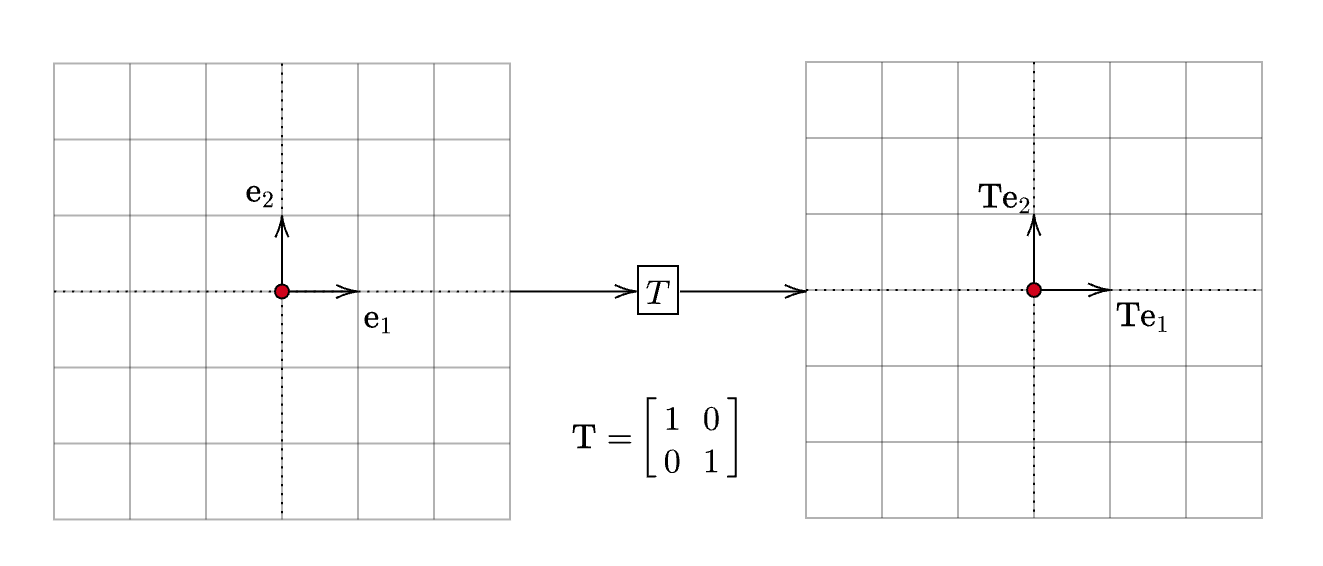
This is not all that interesting. Next:
\[ \mathbf{T} =\begin{bmatrix} 2 & 0\\ 0 & 2 \end{bmatrix} \]
Let us see what this does to the basis vectors:
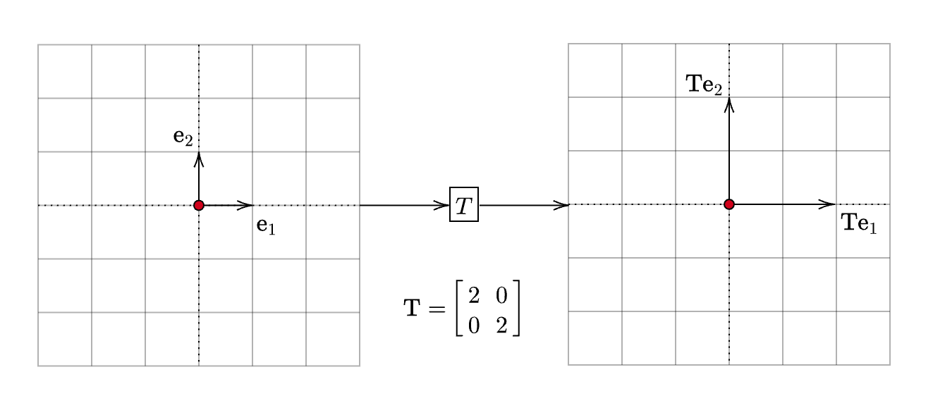
Notice the effect it has. Each vector is scaled. In this case, it is stretched. It becomes twice as long as the input. To see why this is true algebraically, consider an arbitrary vector \(x=\begin{bmatrix} x_{1} & x_{2} \end{bmatrix}^{T}\):
\[ \mathbf{Tx} =\begin{bmatrix} 2 & 0\\ 0 & 2 \end{bmatrix}\begin{bmatrix} x_{1}\\ x_{2} \end{bmatrix} =2\cdot \begin{bmatrix} x_{1}\\ x_{2} \end{bmatrix} =2\mathbf{x} \]
Let us now consider another matrix:
\[ \mathbf{T} =\begin{bmatrix} 0 & -1\\ 1 & 0 \end{bmatrix} \]
The effect it has on the basis vectors is:
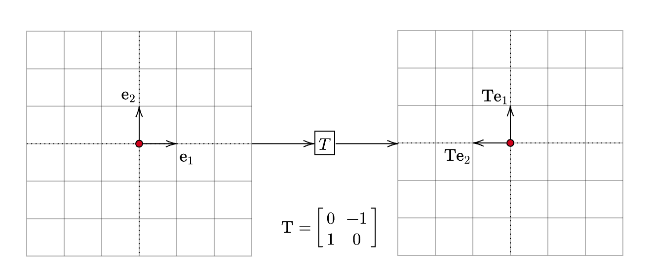
This is a rotation matrix. That is, it rotates the input vector without changing its magnitude. Moving on, let us take up another matrix. This time, let us compose the two linear transformations that we have seen. Composition of linear transformations is equivalent to matrix multiplication:
\[ \mathbf{T} =\begin{bmatrix} 0 & -1\\ 1 & 0 \end{bmatrix}\begin{bmatrix} 2 & 0\\ 0 & 2 \end{bmatrix} =\begin{bmatrix} 0 & -2\\ 2 & 0 \end{bmatrix} \]
What do you expect this matrix to do?
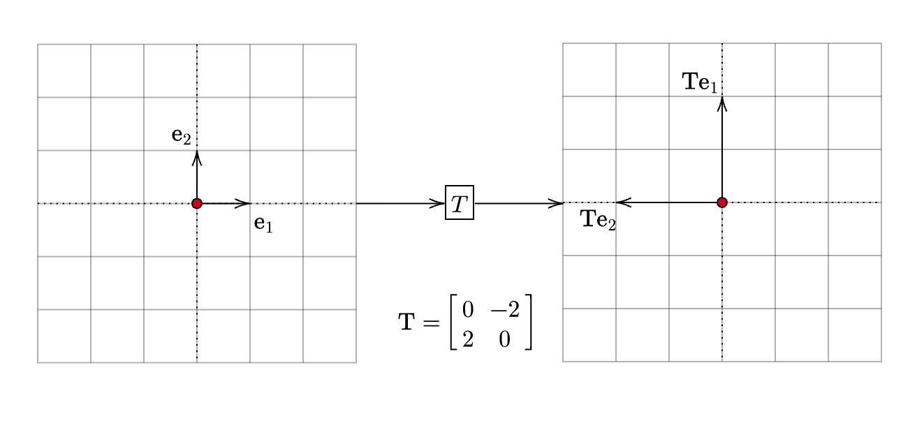
It stretches the vectors and rotates them by \(90^{\circ }\). Note that the two matrices involved in the product are commutative. That is, \(\mathbf{T}_{1}\mathbf{T}_{2} =\mathbf{T}_{2}\mathbf{T}_{1}\). Intuitively, we can see why this is true. We could either stretch a vector and then rotate it (OR) we could rotate it and then stretch it. However, this (commutativity) is not true of any two arbitrary linear transformations. Let us now move to a more complex linear transformation:
\[ \mathbf{T} =\begin{bmatrix} 2 & 1\\ 1 & 2 \end{bmatrix} \]
The effect on basis vectors is:

This is not simple rotation or stretching. It is an example of a shear transformation. Finally, consider the following linear transformation. Let us use the inverse of the matrix we just worked with.
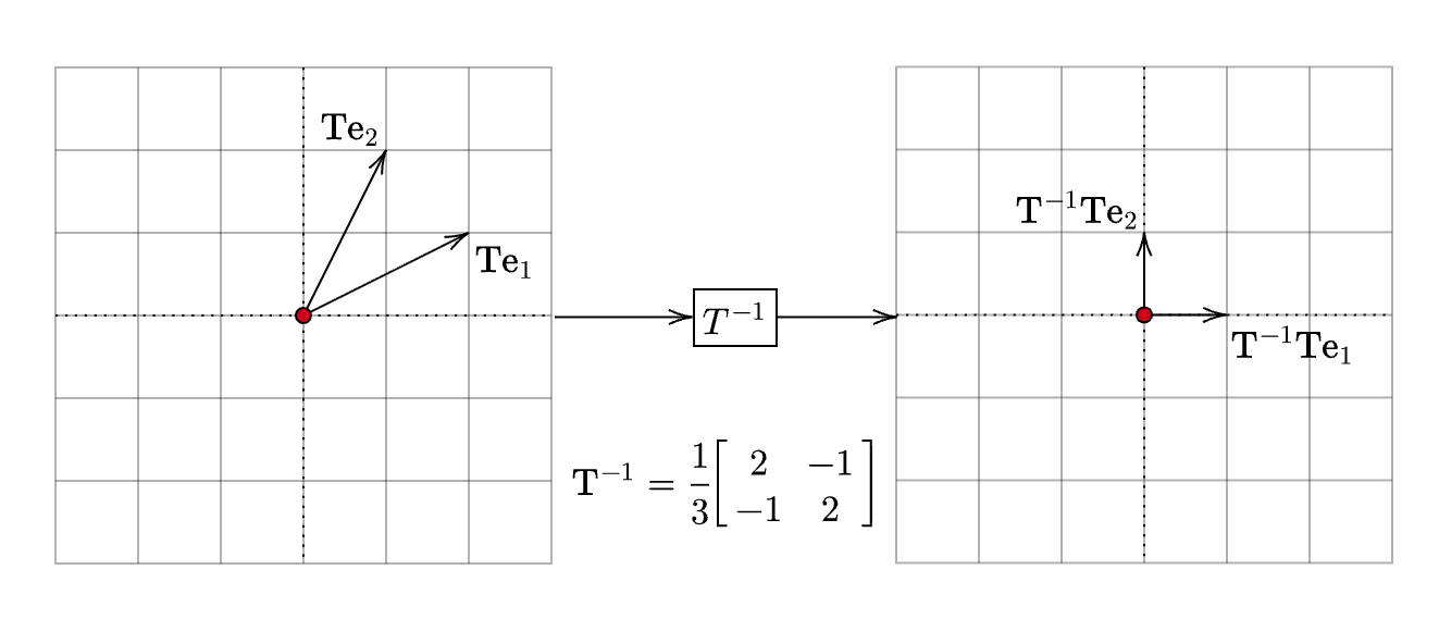
\[ \mathbf{T}^{-1} =\frac{1}{3}\begin{bmatrix} 2 & -1\\ -1 & 2 \end{bmatrix} \]
Now, instead of working with the standard basis, let us see what it does to the vectors \(\displaystyle \{\mathbf{Te}_{1} ,\mathbf{Te}_{2}\}\).
Notice that we have:
\[ \begin{aligned} \mathbf{T}^{-1}\mathbf{Te}_{1} & =\mathbf{e}_{1}\\ \mathbf{T}^{-1}\mathbf{Te}_{2} & =\mathbf{e}_{2} \end{aligned} \]
When \(\displaystyle \mathbf{T}^{-1}\) acts on \(\displaystyle \mathbf{Te}_{1} ,\mathbf{Te}_{2}\), it does the reverse action by taking them back to their parents \(\displaystyle \mathbf{e}_{1} ,\mathbf{e}_{2}\). Algebraically, this shows that \(\displaystyle \mathbf{T}^{-1}\mathbf{T} =\mathbf{I}\), the identity matrix which corresponds to the identity transformation.
Now that we have a good idea of what linear transformations do, we are ready to explore the idea of eigenvalues and eigenvectors.
Summary
Linear transformations are functions between vector spaces that preserve linearity. A linear transformation is completely determined by its action on the basis vectors in the domain. Each linear transformation can be represented as a matrix and vice-versa. A composition of linear transformations is equivalent to matrix multiplication between the corresponding matrices representing them.